Atomic Density¶

Density Analysis¶

Understanding the positions of atoms in a material is incredibly useful when studying things like atomic structure and defect segregation. Consider a system with an interface, it may be interesting to know how the distributions of the materials atoms change at that interface, e.g is there an increase or decrease in the amount of a certain species at the interface and does this inform you about any segregation behaviour?

This module of polypy allows the positions of atoms in a simulation to be evaluated in one and two dimensions, this can then be converted into a charge density and (in one dimension) the electric field and electrostatic potential.

from polypy.read import History
from polypy.read import Archive
from polypy.density import Density
from polypy import analysis
from polypy import utils as ut
from polypy import plotting

import numpy as np
import matplotlib.pyplot as plt
import warnings
warnings.filterwarnings('ignore')

In this tutorial, we will use polypy to analyse a molecular dynamics simulation of a grain boundary in fluorite cerium oxide and a Monte Carlo simulation of Al, Li and Li vacancy swaps in lithium lanthanum titanate.

Example 1 - Cerium Oxide Grain Boundary¶

In this example we will use polypy to analyse a molecular dynamics simulation of a grain boundary in cerium oxide.

The first step is to read the data. We want the data for both species so need to provide a list of the species.

["CE", "O"]

Note. In all examples, an xlim has been specified to highlight the grain boundary. Feel free to remove the ax.set_xlim(42, 82) to see the whole plot.

history = History("../example_data/HISTORY_GB", ["CE", "O"])

print(np.amin(history.trajectory.cartesian_trajectory))
print(np.amax(history.trajectory.fractional_trajectory))

-63.929
0.9999993486383602

The next step is to create the density object for both species. In this example we create a seperate object for the cerium and oxygen atoms and we will be analysing the positions to a resolution of 0.1 angstroms.

ce_density = Density(history.trajectory, atom="CE", histogram_size=0.1)
o_density = Density(history.trajectory, atom="O", histogram_size=0.1)

All subsequent analysis is performed on these two objects.

One Dimension¶

The one_dimensional_density function will take a direction which corresponds to a dimension of the simulation cell. For example, ‘x’ corresponds to the first lattice vector. The code will calculate the total number of a species in 0.1 angstrom histograms along the first cell dimension.

The function will return the positions of the histograms and the total number of species. These can then be plotted with the one_dimensional_density_plot function which takes a list of histogram values, a list of particle densities and a list of labels.

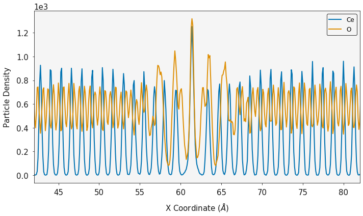
cx, cy, c_volume = ce_density.one_dimensional_density(direction="z")
ox, oy, o_volume = o_density.one_dimensional_density(direction="z")

ax = plotting.one_dimensional_density_plot([cx, ox], [cy, oy], ["Ce", "O"])
ax.set_xlim(42, 82)
plt.show()

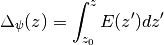
The particle densities can be combined with the atom charges to generate the one dimensional charge density according to

$\rho_q(z) = \sum_{i} q_i \rho_i(z)$

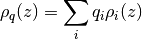
where $\rho_{i}$ is the particle density of atom i and $q_{i}$ is its charge.

The OneDimensionalChargeDensity class is used for the charge density, electric field and electrostatic potential. It requires a list of particle densities, list of charges, the histogram volume and the total number of timesteps.

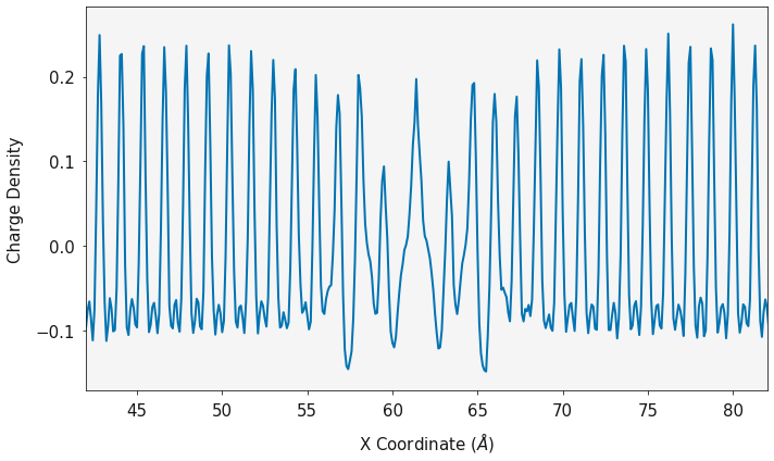
charge = analysis.OneDimensionalChargeDensity(ox, [oy, cy], [-2.0, 4.0], c_volume, history.trajectory.timesteps)

dx, charge_density = charge.calculate_charge_density()

ax = plotting.one_dimensional_charge_density_plot(dx, charge_density)
ax.set_xlim(42, 82)

plt.show()

The charge density can be converted into the electric field and the electrostatic potential.

$E(z) = \frac{1}{- \epsilon_{0}} \int_{z_{0}}^{z} \rho_{q}(z')dz'$

$\Delta_{\psi}(z) = \int_{z_{0}}^{z} E(z')dz'$

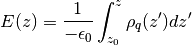
where $\rho_{i}$ is the charge density and $\epsilon_{0}$ is the permittivity of free space The calculate_electric_field and calculate_electrostatic_potential functions will return the electric field and the electrostatic potential.

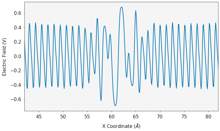
dx, electric_field = charge.calculate_electric_field()

ax = plotting.electric_field_plot(dx, electric_field)
ax.set_xlim(42, 82)
plt.show()

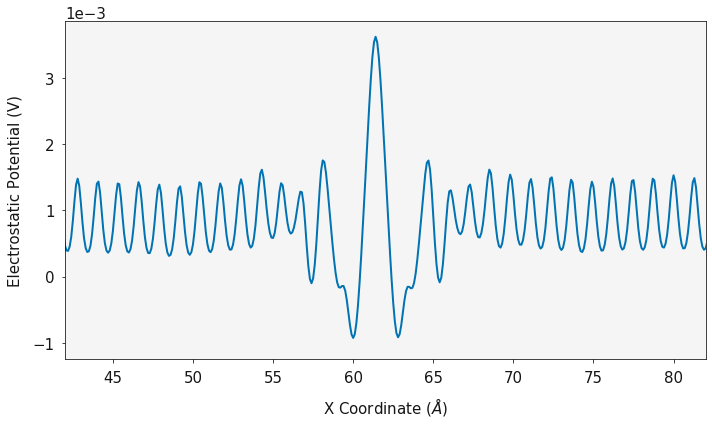
dx, electrostatic_potential = charge.calculate_electrostatic_potential()

ax = plotting.electrostatic_potential_plot(dx, electrostatic_potential)
ax.set_xlim(42, 82)

plt.show()

Two Dimensions¶

The particle density can be evaluated in two dimensions. The two_dimensional_density function will calculate the total number of species in histograms. The coordinates in x and y of the box are returned and a grid of species counts are returned.

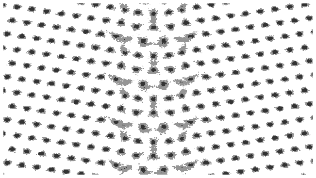
In this example, the colorbar has been turned off, we are using a grey palette and the data is being plotted on a log scale.

cx_2d, cy_2d, cz_2d, c_volume = ce_density.two_dimensional_density(direction="x")
ox_2d, oy_2d, oz_2d, o_volume = o_density.two_dimensional_density(direction="x")

fig, ax = plotting.two_dimensional_density_plot(cx_2d, cy_2d, cz_2d, colorbar=False, palette="Greys", log=True)
ax.set_xlim(42, 82)
ax.axis('off')
plt.show()

fig, ax = plotting.two_dimensional_density_plot(ox_2d, oy_2d, oz_2d, colorbar=False, palette="Greys", log=True)
ax.set_xlim(42, 82)
ax.axis('off')
plt.show()

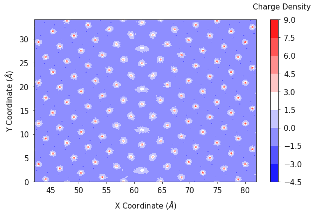
In the same fashion as the one dimensional case, the charge density can be evaluated in two dimensions using the two_dimensional_charge_density function. This function requires the two dimensional array of atom positions, the atom charges, the volume at each grid point and the total number of timesteps in the simulation.

charge_density = analysis.two_dimensional_charge_density([oz_2d, cz_2d], [-2.0, 4.0], o_volume, history.trajectory.timesteps)

fig, ax = plotting.two_dimensional_charge_density_plot(ox_2d, oy_2d, charge_density, palette='bwr')
ax.set_xlim(42, 82)
plt.show()

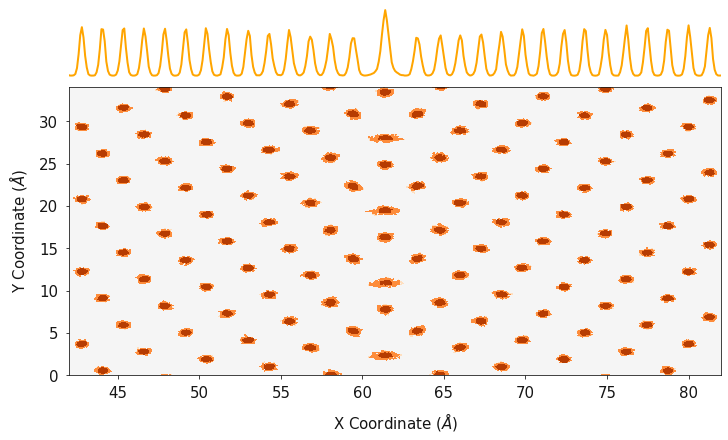
One and Two Dimensions¶

The contour plots can give a good understanding of the average positions of the atoms (or the location of the lattice sites) however it does not give a good representation of how many species are actually there. The combined_density_plot function will evaluate the particle density in one and two dimensions and then overlay the two on to a single plot, allowing both the lattice sites, and total density to be viewed.

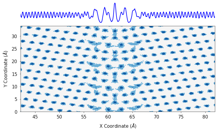
In this example we are using an orange palette and orange line color for the cerium atoms, a blue palette and blue line for the oxygen positions and the data is plotted on a log scale.

fig, ax = plotting.combined_density_plot(cx_2d, cy_2d, cz_2d, palette="Oranges", linecolor="orange", log=True)
for axes in ax:
    axes.set_xlim(42, 82)
plt.show()

fig, ax = plotting.combined_density_plot(ox_2d, oy_2d, oz_2d, palette="Blues", linecolor="blue", log=True)
for axes in ax:
    axes.set_xlim(42, 82)
plt.show()

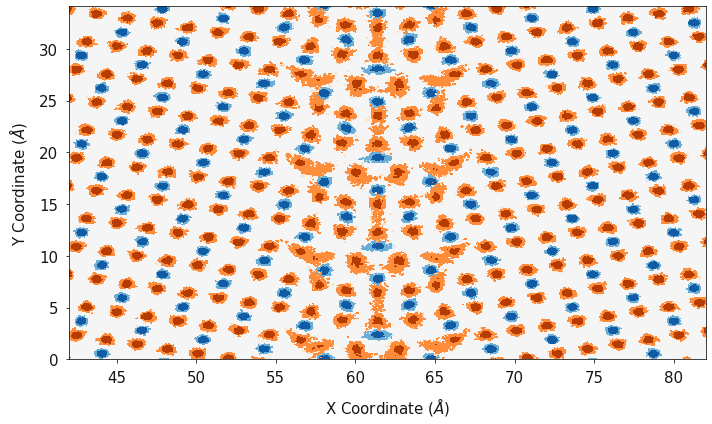
Finally, polypy.plotting has some functions that will generate a single contour plot for all species. This function requires the a list of x axes, a list of y axes, a list of two dimensional arrays corresponding to the x and y axes and a list of color palettes.

fig, ax = plotting.two_dimensional_density_plot_multiple_species([cx_2d, ox_2d], [cy_2d, oy_2d],
                                                                 [cz_2d, oz_2d], ["Blues", "Oranges"],
                                                                 log=True)
ax.set_xlim(42, 82)
plt.show()

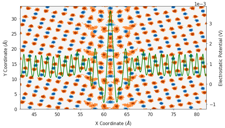
When analysing things like the electrostatic potential, it is useful to be able to view how the electrostatic potential changes with structure, it is very easy to use the polypy.plotting functions in conjunction with matplotlib to visualise the relationships.

fig, ax = plotting.two_dimensional_density_plot_multiple_species([cx_2d, ox_2d], [cy_2d, oy_2d],
                                                                 [cz_2d, oz_2d], ["Blues", "Oranges"],
                                                                 log=True)
ax.set_xlim(42, 82)
ax2 = ax.twinx()
ax2.plot(dx, electrostatic_potential, color="green")
ax2.set_ylabel("Electrostatic Potential (V)")
plt.show()

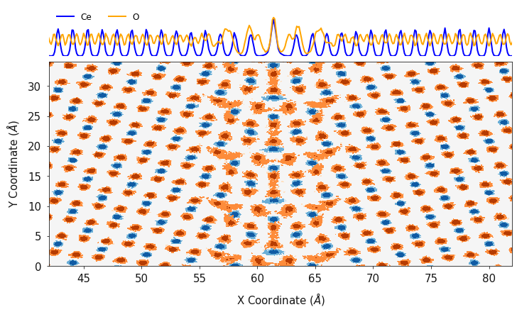
Finally, polypy.plotting can generate a contour plot showing the number density in one and two dimensions in a single plot. This function requires the a list of x axes, a list of y axes, a list of two dimensional arrays corresponding to the x and y axes, a list of color palettes, a list of labels and a list of line colors.

fig, ax = plotting.combined_density_plot_multiple_species(x_list=[cx_2d, ox_2d],
                                                          y_list=[cy_2d, oy_2d],
                                                          z_list=[cz_2d, oz_2d],
                                                          palette_list=["Blues", "Oranges"],
                                                          label_list=['Ce', 'O'],
                                                          color_list=["blue", "orange"],
                                                          log=True)
for axes in ax:
    axes.set_xlim(42, 82)
plt.show()

Example 2 - Li, Al and Li vacancy swaps¶

In this example we will analyse a Monte Carlo simulation of Al doped lithium lanthanum titanate. It is possible to use molecular dynamics simulations to study defect segregation if the defects have a relatively high diffusion coefficient. One could randomly dope a configuration, run a long molecular dynamics simulation and then analyse the evolution of the defect locations. When the diffusion coefficient of your defect is very low, it is not possible to use molecular dynamics simulations to study defect segregation because you would need a huge MD simulation, in order to record enough statistics. Monte Carlo simulations allow you to perform unphysical moves and with a comparitively small Monte Carlo simulation, you can generate enough statistics to reliably study things like defect segregation.

In this example, we are analysing a MC simulation of Al in LLZO. $Al^{3+}$ has been doped on the $Li^{+}$ sites and charge compensating Li vacancies have been added. Ultimately, we want to calculate how the Al doping effects the Li conductivity, however without a representative distribution of Al/Li/Li vacancies we can’t calculate a representative conductivity. After 10 ns of MD, the distribution of Al was unchanged, so Monte Carlo simulations with swap moves are needed to shake up the distribution. The following swap moves were used;

Al <-> Li
Al <-> $V_{Li}$
Li <-> $V_{Li}$

ARCHIVE_LLZO is a short MC trajectory that we will analyse.

First we will extract and plot the configuration at the first timestep and then we will plot the positions across the whole simulation to see how the distributions have changed.

archive = Archive("../example_data/ARCHIVE_LLZO", ["LI", "AL", "LV"])
config_1 = archive.trajectory.get_config(1)

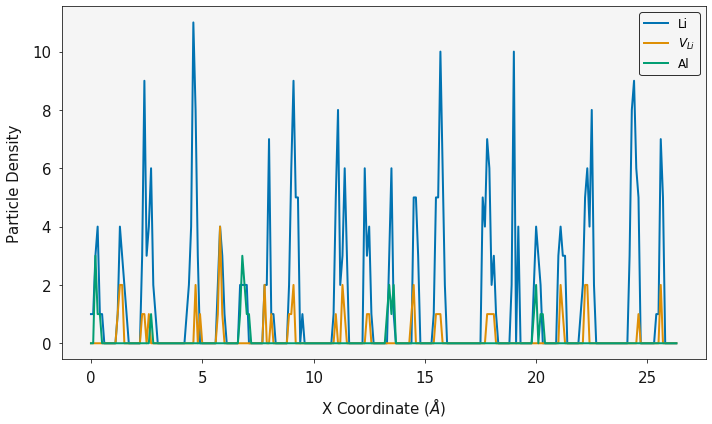
Timestep 1¶

li_density = Density(config_1, atom="LI", histogram_size=0.1)
al_density = Density(config_1, atom="AL", histogram_size=0.1)
lv_density = Density(config_1, atom="LV", histogram_size=0.1)

lix, liy, li_volume = li_density.one_dimensional_density(direction="y")
alx, aly, al_volume = al_density.one_dimensional_density(direction="y")
lvx, lvy, lv_volume = lv_density.one_dimensional_density(direction="y")

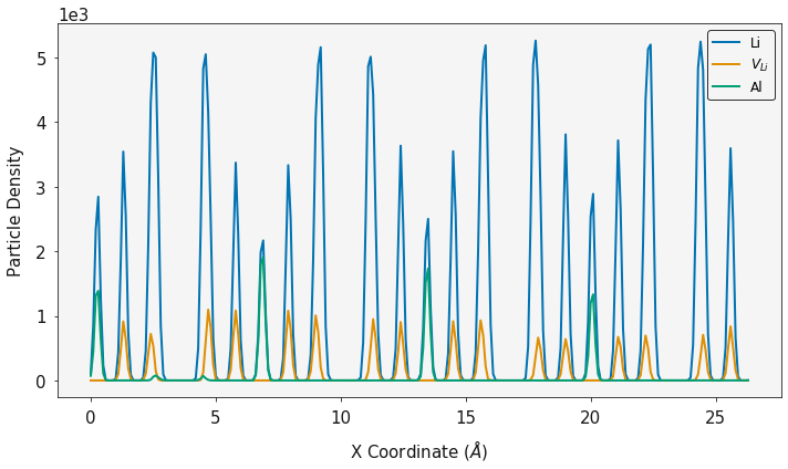
ax = plotting.one_dimensional_density_plot([lix, lvx, alx], [liy, lvy, aly], ["Li", "$V_{Li}$", "Al"])
plt.show()

Full Simulation¶

Disclaimer. This is a short snapshot of a simulation and is not fully equilibriated, however it provides an example of the polypy functionailty.

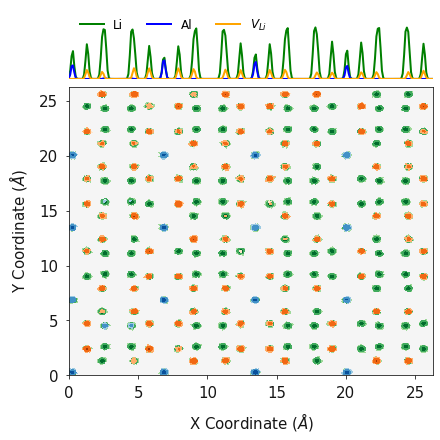
Interestingly, what we find is that the Al, Li and $V_{Li}$ tend to distribute in an even pattern within the structure. This is in sharp contrast to the distribution at the start of the simulation.

li_density = Density(archive.trajectory, atom="LI", histogram_size=0.1)
al_density = Density(archive.trajectory, atom="AL", histogram_size=0.1)
lv_density = Density(archive.trajectory, atom="LV", histogram_size=0.1)

lix, liy, li_volume = li_density.one_dimensional_density(direction="y")
alx, aly, al_volume = al_density.one_dimensional_density(direction="y")
lvx, lvy, lv_volume = lv_density.one_dimensional_density(direction="y")

ax = plotting.one_dimensional_density_plot([lix, lvx, alx], [liy, lvy, aly], ["Li", "$V_{Li}$", "Al"])
plt.show()

lix_2d, liy_2d, liz_2d, li_volume = li_density.two_dimensional_density(direction="z")
alx_2d, aly_2d, alz_2d, al_volume = al_density.two_dimensional_density(direction="z")
lvx_2d, lvy_2d, lvz_2d, lv_volume = lv_density.two_dimensional_density(direction="z")

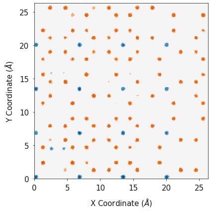
fig, ax = plotting.two_dimensional_density_plot_multiple_species([alx_2d, lvx_2d], [aly_2d, lvy_2d],
                                                                 [alz_2d, lvz_2d], ["Blues", "Oranges"],
                                                                 log=True, figsize=(6, 6))
plt.show()

fig, ax = plotting.combined_density_plot_multiple_species(x_list=[lix_2d, alx_2d, lvx_2d],
                                                          y_list=[liy_2d, aly_2d, lvy_2d],
                                                          z_list=[liz_2d, alz_2d, lvz_2d],
                                                          palette_list=["Greens", "Blues", "Oranges"],
                                                          label_list=["Li", 'Al', '$V_{Li}$'],
                                                          color_list=["green", "blue", "orange"],
                                                          log=True, figsize=(6, 6))
plt.show()